A brief history of Bayesian and frequentist methods
When probability was first studied in the 1800’s (maybe a little earlier), Bayesian methods were the initial ones studied - to Bayes and Laplace and Gauss, it was the natural way to think about things. It became evident that for any reasonable model, however, the calculations were too complex. And thus frequentist statistics (without priors) was born.
Proponents of frequentism are mostly in that camp because that’s the way it’s been done in all science, etc, for a long time. But frequentism never would have had a chance if there had been the computing power we had today back then, and never mind that computers would not have been possible without a lot of science based on frequentist statistics. Frequentists also say that putting a prior on things is bad science.
Why it’s natural
What it really means to have prior information, and why it’s so natural? Even watching how I think has convinced me that even though I was a frequentist by choice, my thinking has always been Bayesian in nature. I’m sure a lot of people think like this: they form an opinion on a subject, even with no knowledge. They get data (learn things) about said subject, and modify their opinion, but it’s always true that the first (prior) opinion affects things. Here “subject” can be anything, such as climate change or who’s the best baseball player.
And science has always had hypotheses before experiments. And the experiment guides the creation of new hypotheses.
Philosophical difference
Bayesian: says the data are fixed, and any parameters (i.e. for height of people as an example, the reason that people of a population are a given height) are random. Best suited to (re)allocate the credibility of a statement.
Frequentist: the data are randomly drawn from a process with a fixed set of population parameters. This is a necessary assumption for frequentist theory. Another necessary assumption is that we can draw samples from that process an infinite number of times. Best suited to falsify a hypothesis.
Consider the question “what is your height?”. For a classical statistician there exists some abstract “true answer”, say “180cm”, which is a fixed number - your one and only height. The problem is, of course, you do not know this number because every measurement is slightly different, so the classical statistician will add that “there is a normally-distributed measurement error”.
In the world of a pure Bayesian there are almost no “fixed numbers” - everything is a probability distribution, and so is your height! That is, a Bayesian should say that “your height is a Normal distribution centered around 180cm”.
The Bayesian approach yields a result of the form: “What is the probability that A is better at converting visitors than B?” which is far more intuitive than “What is the probability that the difference between A and B is under my detection threshold, given the level of false positives and false negatives that I’m ok with?”. Which is somehow much more convoluted.
Note that from the mathematical perspective there is no difference between the two representations - in both cases the number 180cm is mentioned, and the normal distribution. However, from a philosophical, methodological and “mental” perspectives this tends to have serious implications
Example: Truck route
Bayesian “thinking” tends to be more flexible for complex models. Many classical statistics models would stick to fixed parameters, point or “interval” inferences, and try to “hide” the complexity of probability distributions as much as possible. As a result, reasoning about a system with many highly interconnected concepts becomes flawed. Consider a sequence of three questions:
- What the height of this truck?
- Will it fit under this 3m bridge?
- Do we need pick another route?
In the “classical” mindset you would tend to give fixed answers to the questions.
- “Height of the truck is 297”.
- “Yes, 297 < 300, hence it will fit”.
- “No, we do not need”.
Sometimes you may be more careful and work with confidence intervals, but it still feels unwieldy:
- “The confidence interval on the height of the truck is 290 ~ 310”
- “… aahm, it might not fit…”
- “Let’s pick another route, just in case”
Note, if a followup question appears that depends on the previous inferences (e.g. “do we need to remodel the truck”) answering it becomes even harder because the true uncertainty is “lost” in the intermediate steps.
Such problems are never present if you are disciplined as a Bayesian. Note the answers:
- “The height of the truck is a normal distribution N(297, 10)”
- “It will fit under the bridge with probability of 60%”
- “We need another route with probability of 40%”
At any point is information about the uncertainty is preserved in the distributions and you are free to combine it further, or apply a decision-theoretic utility model. This makes Bayesian networks possible, for example.
So the idea behind Bayesian methods is:
“The data we collected is affected by some parameters so that we try to find the parameters which is limited by our prior knowledge to maximize the chance this data happen”
This is the key different between Bayesian and Frequentist:
- The frequentist get the data and try to generalize that data to the whole population, it’s very human nature.
- You see all your neighbors driving pinky cars => you end up the whole city love pinky cars.
- Instead, Bayesian thinks about some parameters affected the choice of your neighbors.
- You have strong evidence that all your neighbors are young girls. So that why most of the cars are pink.
But what if some guys love driving pinky cars also? This is the risk of Bayesian, if your prior is wrong and the data you have is not big enough, everything goes wrong!
Bayesian Statistics - Big Data
The essence of Bayesian statistics is the combination of information from multiple sources. We call this data and prior information, or hierarchical modeling, or dynamic updating, or partial pooling, but in any case it’s all about putting together data to understand a larger structure. Big data, or data coming from the so-called internet of things, are inherently messy: scraped data not random samples, observational data not randomized experiments, available data not constructed measurements. So statistical modeling is needed to put data from these different sources on a common footing.
Bayesian statistics simply is one branch of statistics that relies on subjective probabilities and Bayes theorem to “update” knowledge regarding events and quantities of interest based on data - in order words, Bayesian statistics can draw/update/alter inferences regarding events/quantities when more data is available. For example, based on some knowledge, we can draw some initial set of inferences regarding the system (referred to as “prior” in Bayesian statistics) and then “update” these inferences based on data (to obtain the so-called “posterior”).
As we can see clearly, there is so much synergy between these two, especially in today’s world where big data and predictive analytics have become so prominent. We have loads and loads of data for variety of systems, and we can constantly make data-driven inferences about the system and keep updating them as more and more data becomes available. Since Bayesian statistics provides a framework for updating knowledge, it is in fact used a whole lot in machine learning.
Bayesian Statistics - Small Data
Let’s say you have a simple upvote capability on your site to upvote Bert and Ernie. Bert has 2 upvotes and 0 downvotes, while Ernie has 45 upvotes and 5 downvotes. A simple frequentist MLE estimate would rank Bert above Ernie, as Bert has 100% upvotes, while Ernie has only 90% upvotes. This unfair to Ernie as Bert barely has any respondants.
What we can do is attach a prior to Bert and Ernie This would be equivalent to giving them some upvotes and downvotes even before we start collecting user data. We can give each 1 upvote and 1 downvote (this is equivalent to placing a flat Beta(1,1) prior on your distribution of what their true proportion upvotes should be). Now Bert will have 3 upvotes and 1 downvote while Ernie will have 46 upvotes and 6 downvotes. Bert will now be 75% upvotes while Ernie will be 88% upvotes. We will now rank Ernie above Bert.
Problem - Baseball batting average
Anyone who follows baseball is familiar with batting averages- simply the number of times a player gets a base hit divided by the number of times he goes up at bat (so it’s just a percentage between 0 and 1). 0.266 is in general considered an average batting average, while 0.300 is considered an excellent one.
Imagine we have a baseball player, and we want to predict what his season-long batting average will be. You might say we can just use his batting average so far- but this will be a very poor measure at the start of a season! If a player goes up to bat once and gets a single, his batting average is briefly 1.000, while if he strikes out or walks, his batting average is 0.000. It doesn’t get much better if you go up to bat five or six times- you could get a lucky streak and get an average of 1.000, or an unlucky streak and get an average of 0, neither of which are a remotely good predictor of how you will bat that season.
Why is your batting average in the first few hits not a good predictor of your eventual batting average? When a player’s first at-bat is a strikeout, why does no one predict that he’ll never get a hit all season? Because we’re going in with prior expectations. We know that in history, most batting averages over a season have hovered between something like 0.215 and 0.360, with some extremely rare exceptions on either side. We know that if a player gets a few strikeouts in a row at the start, that might indicate he’ll end up a bit worse than average, but we know he probably won’t deviate from that range.
Given our batting average problem, which can be represented with a binomial distribution (a series of successes and failures), the best way to represent these prior expectations is with the beta distribution. It’s saying, before we’ve seen the player take his first swing, what we roughly expect his batting average to be.
We expect that the player’s season-long batting average will be most likely around 0.27, but that it could reasonably range from 0.21 to 0.35. This can be represented with a beta distribution with parameters \(\alpha=81\) and \( \beta=219\):
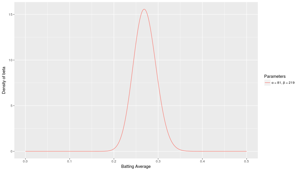
I came up with these parameters for two reasons:
-
The mean is \(\frac{\alpha}{\alpha + \beta} = \frac{81}{81+219} = 0.270\)
-
As you can see in the plot, this distribution lies almost entirely within \((0.2,.35)\) - the reasonable range for a batting average.
Here’s why the beta distribution is so appropriate. Imagine the player gets a single hit. His record for the season is now “1 hit; 1 at bat.” We have to then update our probabilities- we want to shift this entire curve over just a bit to reflect our new information. While the math for proving this is a bit involved (it’s shown here), the result is very simple. The new beta distribution will be:
\[\mbox{Beta}(\alpha_0+\mbox{hits}, \beta_0+\mbox{misses})\]The more the player hits over the course of the season, the more the curve will shift to accommodate the new evidence, and furthermore the more it will narrow based on the fact that we have more proof. Let’s say halfway through the season he has been up to bat 300 times, hitting 100 out of those times. The new distribution would be \(\mbox{beta}(81+100, 219+200)\):
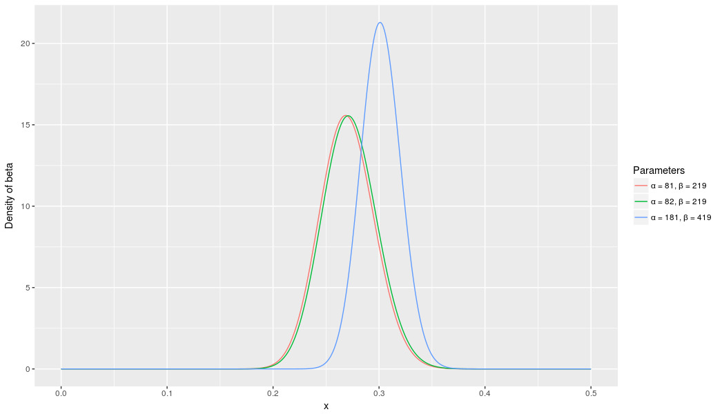
Notice the curve is now both thinner and shifted to the right (higher batting average) than it used to be- we have a better sense of what the player’s batting average is.
One of the most interesting outputs of this formula is the expected value of the resulting beta distribution, which is basically your new estimate. Recall that the expected value of the beta distribution is \(\frac{\alpha}{\alpha+\beta}\). Thus, after 100 hits of 300 real at-bats, the expected value of the new beta distribution is \(\frac{82+100}{82+100+219+200}=.303\). You might notice that this formula is equivalent to adding a “head start” to the number of hits and non-hits of a player- you’re saying “start him off in the season with 81 hits and 219 non hits on his record”).
Thus, the beta distribution is best for representing a probabilistic distribution of probabilities- the case where we don’t know what a probability is in advance, but we have some reasonable guesses.
More about it
- The baseball analysis was based on David Robinson’s post. Looking for more? It brings a lot of valuable posts on Bayesian analysis! Have a look on his website.
- A great hands on to understand the Bayesian thinking Beginning Bayes - Datacamp