Visualization with R
This post will be a simple analysis on electoral data from Brazil. I’ll explore some points at the data and draw beautiful plots using ggplot package. I hope you enjoy the potential of R to make informative and clean graphs.
knitr::opts_chunk$set(echo = TRUE)
library(dplyr)
library(data.table)
library(magrittr)

library(ggplot2)
library(scales)
library(extrafont)

library(RCurl)
A brief explain on the packages:
- dplyr and data.table are the undispensible tools for every analysis.
- ggplot2, scales and extrafont are the best tools for static plots.
- Rcurl is good workaround package to solve download issues.
Before going further, let’s get a single file and have a overall look on it. The candidates file of electoral race can be downloaded from the Superior Electoral Court website.
tf <- tempfile(); td <- tempdir()
url = 'http://agencia.tse.jus.br/estatistica/sead/odsele/consulta_cand/consulta_cand_2016.zip'
download.file(url, destfile = tf)
unzip(tf, exdir = td)
The system R function calls a bash command. Let’s use them to have a look on the files. The system function have a different way of outputting the results. This is a problem that can easily be overcome by a little hacking.
# To capture the bash output
system = function(...) cat(base::system(..., intern = TRUE), sep = "\n")
# Filesize
system(sprintf('cd %s; wc -c consulta_cand_2016_SP.txt', td))
## 46096775 consulta_cand_2016_SP.txt# Head
system(sprintf('cd %s ;
head -n 3 consulta_cand_2016_SP.txt | iconv -f iso-8859-1 -t UTF-8', td))## "12/11/2016";"19:17:15";"2016";"1";"Eleições Municipais 2016";"SP";"65714";"ITATINGA";"13";"VEREADOR";"LUZIA MARIA CARLOS ROSA";"250000004564";"25000";"04000800876";"LUZIA";"2";"DEFERIDO";"25";"DEM";"DEMOCRATAS";"250000000243";"#NULO#";"PMDB / DEM";"PMDB - DEM";"922";"SERVIDOR PÚBLICO CIVIL APOSENTADO";"28/06/1959";"015319110132";"57";"4";"FEMININO";"8";"SUPERIOR COMPLETO";"3";"CASADO(A)";"01";"BRANCA";"1";"BRASILEIRA NATA";"SP";"-3";"SÃO MANUEL";"0";"4";"NÃO ELEITO";"ACA_CORE@HOTMAIL.COM"
## "12/11/2016";"19:17:15";"2016";"1";"Eleições Municipais 2016";"SP";"65358";"ITABERÁ";"13";"VEREADOR";"JOEL ANTONIO LEANDRO";"250000004674";"12500";"11235818861";"JOEL LEANDRO";"2";"DEFERIDO";"12";"PDT";"PARTIDO DEMOCRÁTICO TRABALHISTA";"250000000252";"#NULO#";"PDT / PRP";"'PDT/PRP'";"606";"TRABALHADOR RURAL";"11/05/1968";"022687330159";"48";"2";"MASCULINO";"3";"ENSINO FUNDAMENTAL INCOMPLETO";"3";"CASADO(A)";"01";"BRANCA";"1";"BRASILEIRA NATA";"SP";"-3";"ITABERA";"-1";"5";"SUPLENTE";"AMEITABERA@HOTMAIL.COM"
## "12/11/2016";"19:17:15";"2016";"1";"Eleições Municipais 2016";"SP";"66419";"LINDÓIA";"13";"VEREADOR";"LUCIMARA GODOY DO CARMO GENEROSO";"250000016232";"12222";"15279204889";"LUCIMARA GODOY";"2";"DEFERIDO";"12";"PDT";"PARTIDO DEMOCRÁTICO TRABALHISTA";"250000000982";"#NULO#";"PDT / SD / PMDB";"SOMOS TODOS LINDÓIA";"117";"FARMACÊUTICO";"20/06/1973";"191031290116";"43";"4";"FEMININO";"8";"SUPERIOR COMPLETO";"3";"CASADO(A)";"01";"BRANCA";"1";"BRASILEIRA NATA";"SP";"-3";"SERRA NEGRA";"0";"5";"SUPLENTE";"MARAGODOYGENEROSO@HOTMAIL.COM"The, likely, biggest file have only 46 Mb. The file does not have a header, the NULL entries are “#NULO#” and the separator is ”;”. The year states files come with a README pdf. There you can see the header.
The next step is do it in a loop so I can have candidates files candidates file for the 2004 year until 2016. As the files comes separeted by states, we have to bind them into one. It can be done in R, but it’s easier and faster in bash using cat.
Fortunately I found a Github repository that have mapped the header - Github silvadenisson. I saved the naming part of the file in my Github. Know, let’s use it.
Downloading and transforming the raw data
candidates_data <- list()
# Load the function that brings the correct header
eval(expr =
       parse(text = getURL("https://raw.githubusercontent.com/MatheusRabetti/matheusrabetti.github.io/master/assets/posts/candidates-beautiful-plot/header.R",
                           ssl.verifypeer=FALSE) ))

for(ano in seq(2004, 2016, 4)){
  cat('Downloading year', ano, '\n')

  # Download and save in a temporary folder
  sprintf('http://agencia.tse.jus.br/estatistica/sead/odsele/consulta_cand/consulta_cand_%s.zip',ano) %>%
    download.file(destfile = tf, quiet = T)
  unzip(tf, exdir = td)

  cat('Binding and reading the files ...\n')
  # Binding
  system(sprintf('cd %s; cat consulta*%s*.txt >> all-%s.txt', td, ano, ano))
  # Reading
  candidates_data[[as.character(ano)]] <-
    fread(sprintf('%s/all-%s.txt',td,ano),
          header = F, sep = ";",
          stringsAsFactors = F,
          encoding = "Latin-1")


  candidates_header(candidates_data[[as.character(ano)]])

}
## Downloading year 2004
## Binding and reading the files ...
##
##
Read 39.8% of 401789 rows
Read 59.7% of 401789 rows
Read 82.1% of 401789 rows
Read 401789 rows and 43 (of 43) columns from 0.171 GB file in 00:00:06
## Downloading year 2008
## Binding and reading the files ...
##
##
Read 44.2% of 384532 rows
Read 62.4% of 384532 rows
Read 98.8% of 384532 rows
Read 384532 rows and 43 (of 43) columns from 0.162 GB file in 00:00:05
## Downloading year 2012
## Binding and reading the files ...
##
##
Read 4.1% of 483825 rows
Read 35.1% of 483825 rows
Read 66.1% of 483825 rows
Read 95.1% of 483825 rows
Read 99.2% of 483825 rows
Read 483825 rows and 44 (of 44) columns from 0.231 GB file in 00:00:09
## Downloading year 2016
## Binding and reading the files ...
##
##
Read 40.2% of 497125 rows
Read 42.2% of 497125 rows
Read 70.4% of 497125 rows
Read 98.6% of 497125 rows
Read 497125 rows and 46 (of 46) columns from 0.251 GB file in 00:00:08candidates_data <- data.table::rbindlist(candidates_data, use.names = T, fill = T)I’ll select the variables listed below to continue my analysis:
- ANO_ELEICAO: Election year
- DESCRICAO_CARGO: Description of the position that the candidate runs for.
- DESCRICAO_OCUPACAO: Candidate’s occupation description.
- CODIGO_SEXO: Candidate’s sex code.
- DESCRICAO_SEXO: Candidate’s sex description.
At first I want to see the percentage of women that canditates in politics in Brazil. So, let’s use dplyr to manipulte the data.
table(candidates_data$CODIGO_SEXO)##
## 0 2 4
## 209 1288863 478199candidates_data %>%
select(ANO_ELEICAO, DESCRICAO_CARGO, DESCRICAO_OCUPACAO,
CODIGO_SEXO, DESCRICAO_SEXO) %>%
filter(CODIGO_SEXO %in% c(2,4)) %>%
group_by(ANO_ELEICAO) %>%
summarise(fem_percent = round(sum(CODIGO_SEXO == '4')/n(), 4)) %>%
mutate(xtralabs = ifelse(fem_percent == max(fem_percent), 'Highest:\n',
ifelse(fem_percent == min(fem_percent), 'Lowest:\n',''))) -> female_percent
knitr::kable(female_percent)| ANO_ELEICAO | fem_percent | xtralabs |
|---|---|---|
| 2004 | 0.2125 | Lowest: |
| 2008 | 0.2129 | |
| 2012 | 0.3152 | |
| 2016 | 0.3188 | Highest: |
Analysis - drawing a portrait of electoral candidates
Before you run the next command I advise you install de extrafont package, indispensable if you use Linux. The font you use in a plot absolutely changes the view of it. This package helps you administrates your fonts and even install new.
female_percent %>%
  ggplot(., aes(ANO_ELEICAO, fem_percent)) +
  geom_bar(stat = 'identity', width = .65) +
  geom_label(aes(label = sprintf('%s%s', xtralabs, percent(fem_percent))),
             vjust = -.4,
             family= rep("Verdana", 4),
             fontface = c('bold', rep('plain',3)),
             lineheight=.9, size=4, label.size = 0) +
  scale_x_discrete() +
  scale_y_continuous(expand = c(0,0), limits = c(0.0,1.0), labels = percent) +
  labs(x=NULL, y=NULL, title="Portrait of Brazilian Politics",
       captions = 'Data from TSE/Repositório Eleitoral',
       subtitle = 'Female percentage of electoral candidacy') +
  theme_minimal(base_family = 'Verdana') +
  theme(axis.line = element_line(color='#2b2b2b', size =.5) ) +
  theme(axis.line.y = element_blank()) +
  theme(axis.text.x = element_text(family = rep("Verdana", 4),
                                   face = c('bold', rep('plain', 3)))) +
  theme(panel.grid.major.x=element_blank()) +
  theme(panel.grid.major.y=element_line(color="#b2b2b2", size=0.1)) +
  theme(panel.grid.minor.y=element_blank())+
  theme(plot.title=element_text(hjust=0,
                                family="Verdana",
                                face = 'bold',
                                margin=margin(b=10))) +
  theme(plot.caption = element_text(hjust = 0,
                                    family = 'Verdana',
                                    margin = margin(t = 20))) +
  theme(plot.subtitle = element_text(margin = margin(b = 20),
                                     family = 'Verdana'))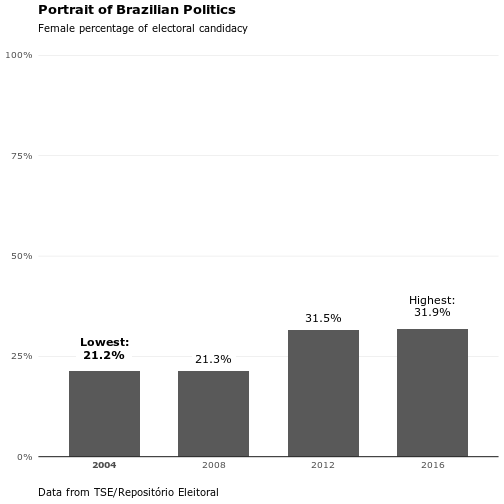
The situation is getting better, but is far from being considered good. There is still a gap of 18.1% to the ideal cenary of half of candidates.